
4.1 Digital Imagery

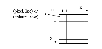
Each picture element in an image, called a pixel, has coordinates of (x, y) in the discrete space representing a continuous sampling of the earth surface. Image pixel values represent the sampling of the surface radiance. Pixel value is also called image intensity, image brightness or grey level. In a multispectral image, a pixel has more than one grey level. Each grey level corresponds to a spectral band. These grey levels can be treated as grey-level vectors.Figure 4.1. An image coordinate system
From the continuous physical space to the discrete image space, a quantization process is needed. The details of quantization is determined by how we do sampling and what kind of resolution we use. General concepts on sampling and resolution have been introduced in Chapter 1.
Two concepts are of particular importance; image space and feature space. Image space refers to the spatial coordinates of an image(s) which are denoted as I with m x n elements, where m and n are respectively the number of rows and the number of columns in the image(s). The elements in image space, I(i,j) (i = 1, 2,..., m; j = 1, 2,..., n) are image pixels. They represent spatial sampling units from which electromagnetic energy or other phenomena are recorded. All possible image pixel values constitute the feature space V. One band of image constitutes a one-dimensional feature space. k bands in an image denoted as Ik construct a k-dimensional feature space Vk. Each element in Vk is a unit hypercube whose coordinate is a k-dimensional vector v = (v1, v2, ..., vk)T. When k = 1, 2, and 3 the hypercube becomes a unit line, a unit area, and a real unit cube. Each pixel in image space has one and only one vector in feature space. Different pixels may have the same vector in feature space.
Multispectral images construct a special feature space, a multispectral space Sk. In S, each unit becomes a grey-level vector g = (g1, g2, ..., gk)T. In multispectral images, each pixel has a grey-level vector. There are other types of images which add additional dimensions to the feature space. In the feature space, various operations can be performed. One of these operations is to classify feature space into groups with similar grey-level vectors, and give each group a same label that has a specific meaning. The classification decision made for each image pixel is in feature space and the classification result is represented in image space. Such an image is a thematic image which could also be used as an additional dimension in feature space for further analysis.
A pixel window is defined in image space as a group of neighbouring pixels. For the computation simplicity, a square pixel neighbourhood wl(i,j) centered at pixel I(i,j) with a window lateral length of l is preferred. Without further explanation, we refer to a pixel window as wl(i,j). In order to ensure that I(i,j) is located at the centre of the pixel window, it is necessary for l to be an odd number. It is obvious that the size of a pixel window wl(i,j) is l X l. The following conditions hold for a pixel window:
![]()
This means that the minimum pixel window is the centre pixel itself, and the maximum pixel window could be the entire image space, provided that the image space is a square with an odd number of rows and columns. When the image space has more than one image, a pixel window can be used to refer to a window located in any one image or any combinations of those images.
A histogram sometimes has two means: a table of occurrence frequencies of all vectors in feature space or a graph plotting these frequencies against all the grey-level vectors. The occurrence frequency in the histogram is the number of pixels in the image segment having the same vector. When the entire image space is used as the image segment, the histogram is referred to as h(I). When a histogram is generated from a specific pixel window, it is identified as hl(i,j) where l, i, and j are the same as above. In practice, one-dimensional feature space is mainly used. In this case, a histogram is a graphical representation of a table with each grey level as an entry of the table. Corresponding to each grey level is its occurrence frequency f(vi) , i = 0, 1, 2, ..., Nv-1 and Nv are the numbers of grey levels of an image (e.g.,Nv = 8 in Figure 4.2).

Figure 4.2. An example histogram
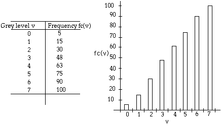
From a histogram h(I) we can derive the cumulative histogram hc(I)={fc(vi) , i = 0, 1, 2, ..., Nv-1}. This is obtained for each grey level by summing up all frequencies whose grey levels are not higher than the particular grey level under consideration (Figure 4.3).

Figure 4.3. A cumulative histogram
In a numerical form that is:
4.1.3 Quality of a Digital Image
Two parameters of a sensor system at a specific height determine the quality of a digital remote sensing image for a given spectral range; the spatial resolution rsand the radiometric resolution rr. As discussed in Chapter 1, the spatial resolution determines how finely the spatial detail of the real world an image can record (i.e., how small the spatial sampling unit is) and therefore the number of pixels in the image space. The radiometric resolution determines how finely a spectral signal can be quantized and therefore the number of grey levels that is produced. The finer these resolutions are, the closer is the information recorded in the image to the real world, and the larger are the sizes of the image space and the grey-level vector space. The size (or alternatively the number of pixels) of image space, S(I), has an exponential relation with the spatial resolution, and so does the size (or the number of vectors) of the feature space, S(V), with the radiometric resolution. Their relations take the following forms:

where k, as defined above, is the number of images in the image space. While S(I) has a fixed exponential order of 2 with rs, S(V) depends not only on rr, but also on k. The number of vectors in Vk becomes extremely large when k grows while rr is unchanged. For example, each band of a Landsat TM or SPOT HRV image is quantized into 8 bits (i.e., an image has 256 possible grey levels). Thus, when k = 1, S(V) = 256 and when k = 3, S(V) = 16,777,216. If a histogram is built in such a three-dimensional multispectral space, it would require at least 64 Megabytes of random access memory (RAM) or disk storage to process it. Therefore, the feature space has to be somehow reduced for certain analyses.
A single image can be represented as a 2-dimensional array. A multispectral image can be represented in a 3-dimensional array (Figure 4.4)
The most popular ones include Band Sequential (BSQ), Pixel Interleaved, Line Interleaved (BIL) or separate files. These format can be illustrated using the following example of a three-band multispectral image.
Figure 4.4. A multispectral image
In a computer, image data can be stored in a number of ways:
AAA BBB CCCBIL is typically used by the Landsat Ground Station Operators' Working Group (LGSOWG)AAA BBB CCC
Band 1 Band 2 Band 3
AAA BBB CCC, AAA BBB CCCBand Sequential BSQ takes the following form:
AAA AAA BBB BBB CCC CCCPixel Interleaved format is used by PCI. It takes the form of:
ABC ABC ABC ABC ABC ABCThese are the general formats that are being used. BIL is suitable for data transfer from the sensor to the ground. It does not need a huge buffer for data storage on the satellite if the ground station is within the transmission coverage of the satellite.
Pixel interleaved is suitable for pixel-based operation or multispectral analysis.
Band sequential and separate
file formats are the proper forms to use when we are more interested in
single-band image processing, such as image matching, correlation, geometric
correction, and when we are more concerned with spatial information processing
and extraction. For example, we use these files when linear features or
image texture are of our concern.