4.5 Image Resampling

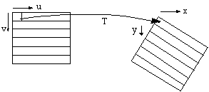
Once the geometric transformation (T) is obtained as we have discussed above, theoretically we can use the following relation to transform each pixel (i,j) from image space (u-v) to a desirable space (x-y).

The results will appear as in Figure 4.13. Pixel position (1, 1) may be transformed to (4850.672, 625.341).

Figure 4.13. Forward transformation results in fractional coordinates in x-y space
In order to have a grid coordinate in x-y space, data have to be resampled in u-v image space for given coordinates in x-y space. This is shown below:

For a pixel location in x-y space, the corresponding coordinates * in u-v space are found through T-1. To determine the grey level at the * location in u-v space, interpolation strategies are used. These include:
ï Nearest neighbour interpolation
ï Bilinear (linear in one dimension)
ï cubic - special case of spline
There are some other interpolation methods, such as use of sinc function, spline function, etc. The most commonly used methods in remote sensing are, however, the three listed above.
Nearest neighbour interpolation simply assigns the value to a pixel that is closest to * as shown below:

In one dimensional case, it can be illustrated as:

This can be achieved using the following convolution operation:

where (u) is the weight function.

One dimensional convolution:

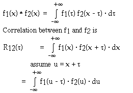
The convolution of two functions f1 and f2 is denoted by,

Convolution is equivalent to flipping filter backwards and then do correlation.
In image enhancement, convolution is the same as correlation since filters are symmetrical.
In image resampling, Id(i) is the discrete image, (i) is the weight function for interpolation
I'(u) = Id(u) * (u)

convolution operator

Since most weight functions are limited to a local neighbourhood, only a limited number of i's need to be used.

For instances, in the nearest neighbour (NN) interpolation, i takes the value which is closest to u. In linear interpretation, l and h takes the nearest integer less than and equal to u and the nearest integer greater than u, respectively. For cubic, l and h takes the second nearest integer less than and equal to u while h takes second closest integer that is greater that u.
For sinc function,

x can be infinite but we usually need to use a limited number of terms up to 20.

According to the above introduction of convolution, for the nearest neighbour case the weight function is

For the linear case, it is

For the cubic convolution:

For the case of two dimension, a sequential process is used.
Z(u) values are first calculated along each row as shown below

Then Z(u, v) is obtained by applying convolution along the dashed line. The convolution process for all the three interpolation cases can be shown by

For the NN, l = m, the closest point to u.

For linear:
l = nearest integer equal or smaller than u
m = nearest integer larger than u

For Cubic:
l = nearest two integers equal or smaller than u
m = nearest two integers larger than u.