6.1 Histogram-Based Operation

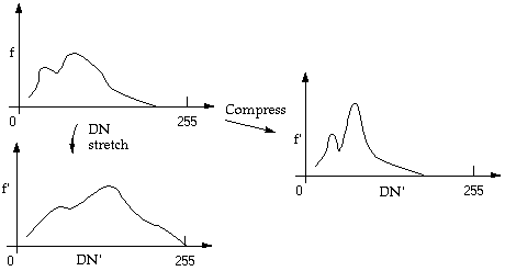
A histogram of an image can tell us about the data distribution with respect to image grey levels. The purpose of a histogram-based operation is that when a grey-level transformation is made, pixels in the image having a specific range of grey levels can be enhanced or suppressed. This is also called contrast adjustment. It can be done using:

1. histogram stretching

2. histogram compression (Figure 6.1)

Figure 6.1. Histogram stretching and compression

Both histogram stretching and histogram compression can be done either linearly or nonlinearly.

a) Linear adjustment (Figure 6.2)

DN' = a ï DN  

 

Figure 6.2.

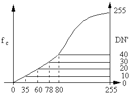
b) Piece-wise linear adjustment (Figure 6.3)

Figure 6.3.

 

From Figure 6.3, we can have The idea of contrast adjustment is the mapping of the range of digital numbers in the original image to a new range. For example, if the image displayed using the histogram in Figure 6.4a appears dark on the screen due to the majority of pixel grey-level values are lower than 150. We can linearly stretch the histogram to transform the grey-level range (0-150) in Figure 6.4a to a new grey-level range (0-255) in Figure 6.4b.

a b

Figure 6.4. (a) original histogram of an image. (b) the histogram after adjustment.

The following transformation can be used:

c) Non-linear adjustment (Figure 6.5)

Figure 6.5. An exponential adjustment  

We can try to use a = 16, b =  , i.e. DN' = 16 .

Other non-linear functions include logarithmic, and even sinusoidal.

d) Non-linear adjustment - histogram equalization

The task of histogram equalization is to transform a histogram of any shape to a histogram which has the same frequency along the whole range of digital number (Figure 6.6).

Figure 6.6. In the continuous case reshape the histogram

This is realized by equally partitioning the cumulative histogram fc of the original image into 255 pieces. Each piece will correspond to one digital number in the equalized image (Figure 6.7). On the cumulative curve, find out the nth dividing point,

DN' = n the corresponding DN is x.

Figure 6.7. For the discrete case, modify the grey level value according to the principle of equal frequency.

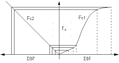
The equalization process can also be considered as a histogram matching method used in image destriping as discussed in Section 5.1. Here we attempt to match the original cumulative histogram Fc1 to the new cumulative histogram Fc2 (Figure 6.8).

Figure 6.8.

The following example shows how an equalization can be made in discrete digital form. It starts with the generation of image histogram (first two columns in Table 6.1). Then probability, Pi is calculated from frequency, f(vi) (third column). A cumulative histogram Fc can be calculated from frequencies. Similarly, the cumulative distribution function (CDF) can be derived from probabilities. Based on the cumulative distribution function we can convert the original grey-levels into grey-levels of the equalized image (Table 2).

Table 6.1 Histogram, cumulative histogram and cumulative distribution function (CDF)

Grey Level (DN)	Frequency f(vi)	Probability Pi	Cumulative histogram Fc	CDF
0	4	0.04	4	0.04
1	17	0.17	21	0.21
2	15	0.15	36	0.36
3	18	0.18	54	0.54
4	24	0.24	78	0.78
5	12	0.12	90	0.90
6	0	0	90	0.90
7	10	0.10	100	1.00
	100	1.00

Table 6.2 Conversion from the grey levels of the
original image to the output image