8.7 Introduction To Neural Networks

Similar to the earlier part of this course, our interests are still focused on the problem that given a piece of evidence e ΠE test the hypothesis that e validates
h ΠH. Transform this into classification or pattern recognition, we would like to have an algorithm or a system that is capable of classifying or recognizing a given set of observations and label it into a class or a pattern. We would like the system or the algorithm learns from observations of patterns that are labelled by class and then is able to recognize unknown patterns and properly label them with output of class membership values.

One of the most exciting developments during the early days of pattern recognition was the perception, the idea that a network of elemental processors arrayed in a manner reminiscent of biological neural nets might be able to learn how to recognize or classify patterns in an autonomous manner. However, it was realized that simple linear networks were inadequate for that purpose and that non-linear networks based on threshold-logic units lacked effective learning algorithms. This problem has been solved by Rumelhart, Hinton and Williams [1986] with a generalized delta rule (GDR) for learning. In the following section, a neural network model based on the generalized delta rule is introduced.

8.7.1. The Generalized Delta Rule For the Semilinear Feed Forward Net With Back Propagation of Error

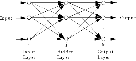
The architecture of a layered net with feed forward capability is shown below:

In this system architecture, the basic elements are nodes "" and links "Æ". Nodes are arranged in layers. Each input node accepts a single value. Each node generates an output value. Depending on the layer that a node is located, its output may be used as the input for all nodes in the next layer.

The links between nodes in successive layers are weight coefficients. For example wji is the link between two nodes from layer i to layer j. Each node is an arithmetic unit. Nodes in the same layer are independent of each other, therefore they can be implemented in parallel processing. Except those nodes of the input layer i, all the nodes take the inputs from all the nodes of the layer and use the linear combination of those input values as its net input, or a node in layer j, the net input is,

uj =  .

The out of the node in layer j is

Oj = f (uj)

where f is the activation function. It often takes the form as a signoidal function,

Oj =  

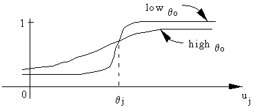
qj serves as a threshold or bias. The effect of a positive qj is to shift the activation function to the left along the horizontal axis. The effect of qo is to modify the shape of the signoid. These effects are illustrated in the following diagram

This function allows for each node to react to certain input differently, some nodes may be easily activated or fined to generate a high output value when qo is low and qj is small. In contrary, when qo is high and qj is large a node will have a slower response to the input uj. This is considered occurring in the human neural system where neurons are activated by different levels of stimuli.

Such a feed forward networks requires a single set of weights and biases that will satisfy all the (input, output) pairs presented to it. The process of obtaining the weights and biases is called network learning or training. In the training task, a pattern  p = {IPi}, i = 1, 2, ..., ni, ni is the number of nodes in the input layer. IP is the input pattern index.

For the given input  p , we require the network adjust the set of weights in all the connecting links and also all the thresholds in the nodes such that the desired outputs  p (= {tpk}, k = 1, 2, ..., nk, nk is the number of output nodes) are obtained at the output nodes. Once this adjustment has been accomplished by the network, another pair of input and output,  p and  p is presented and the network is asked to learn that association also.

In general, the output  p = {Opk} from the network will not be the same as the target or designed values  p. For each pattern, the square of the error is

Ep =  2

and the average system error is

E =  2 .

where the factor of a half is used purely for mathematical convenience at the later stage.

The generalized delta rule (GDR) is used to determine the weights and biases. The correct set of weights is obtained by varying the weights in a manner calculated to reduce the error Ep as rapidly as possible. In general, different results will be obtained depending on one carries out the gradient search in weight space based on either Ep or E.

In GDR, the determination of weights and thresholds is carried out by minimizing Ep.

The convergency of Ep towards improved values for weights and thresholds is achieved by taking incremental changes Æwkj proportional to - _Ep/_wkj . The subscript p will be omitted subsequently, thus

Æwkz = - h   (1)

where E is expressed in terms of outputs Ok, each of which is the non-linear output of the node k,

Ok = f(uk)

where uk is the input to the kth node and it is

uk =   (2)

Therefore by the chain rule,  is evaluated by

 =  ·   (3)

from (2), we obtain

 = Oj (4)

Define

dk = -   (5)

and thus

Æwkj = hdkOj (6)

dk = -  =  ·   (7)

where

 = - (tk - Ok) (8)

and

 = f'k(uk) (9)

Thus

dk = (tk - Ok) f'k(uk) (10)

\ Æwkj = h(tk - Ok) · f'k(uk) · Oj (11)

For weights that do not directly affect output nodes,

Æwji = - h ·  

= - h  ·  

= - h  · Oi

= h  Oi

= h  f'j(uj) · Oi

= h djOi (12)

However  is not directly achievable. Thus it has to be indirectly evaluated in terms of quantities that are known and other quantities that can be evaluated.

-  = -  ·  

=  ·  wkmOm

=  · wkj =  dk · wkj (13)

\ dj = f'j(uj) ·  dk · wkj (14)

That is, the deltas at an internal nodes can be evaluated in terms of the deltas at a later layer. Thus, starting at the last layer, the output layer, we can evaluate dk using equation (10). Then we can propagate the "error" backward to earlier layers. This is the process of error back-propagation.

In summary, with the subscript p denoting the pattern number, we have

Æp wji = h dpj Opi (15)

If the j node is in the output layer,

dpj = (tpj - Opj) · f'j(upj) (16)

If the j node is in internal layers, then

dpj = f'j(upj) ·  · dpk · wkj

Particularly, if

Oj =   (18) 

then

 = Oj(1 - Oj) (19)

and the deltas are

dpk = (tpk - Opk) Opk (1 - Opk)

dpj = Opj (1 - Opj)  · dpk wkj (20)

for the output layer and the hidden layer nodes, respectively.

qj are learned in the same manner as are the other weights.

Note that the number of hidden layer can be greater than 1. Although a three-layer network can form arbitrarily complex decision regions, sometimes difficult learning tasks can be simplified by increasing the number of internal layers. Some preliminary assessment of this algorithm was made for ecological land systems classification of a selected study site in Manitoba (Gong et al., 1994).