5.1 Detector Response Calibration
5.1 Detector Response Calibration
As we have discussed before, Landsat MSS has 6 detectors at each band, TM has 16 and SPOT HRVs have 3000 or 6000 detectors. The differences between the SPOT sensors and Landsat sensors are that each SPOT detector collects one column of an image while each detector of Landsat sensors corresponds to many lines of an image (Figure 5.1).

Figure 5.1. Images acquired using detectors in linear array sensors and in scanners
The problem is that no detector functions the same way as others. If the problem becomes serious, we will observe banding or striping on the image.
There are two types of approach to overcome the detector response problems: absolute calibration and relative calibration.
In this mode, we attempt to establish a relationship between the image grey level and the actual incoming reflectance or the radiation. A reference source is needed for this mode and this source ranges from laboratory light, to on-board light, to the actual ground reflectance or radiation.
For CASI, each detector is calibrated by the manufacturer in the laboratory. For the Landsat MSS, a calibration wedge with 6 different grey levels is used. For the Landsat TM, three lamps, which have 8 brightness combinations, are used.
In any case, a linear response is assumed for each detector
vo = a ï vi + be.g. for an 8-bit image 0 < vo < 255 .vo - observed reading
vi - known source reading
Least squares method is used to derive a and b (Figure 5.2).

Figure 5.2. Responses of the six Landsat
MSS detectors. A least squares linear
fitting is applied to these detector
responses.
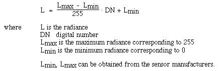
Once each detector is calibrated, the calibrated image data (digital numbers) can be converted into radiances or spectral reflectances. For the case of converting digital numbers of an 8 bit image into radiances, we have
Even though data may have been absolutely calibrated, an image may still have problems caused by sensor malfunctioning. For example, in some of the early Landsat-1, 2, 3 images, there may be lines which have been dropped out. No response for that particular detector can be found. In other cases, there are still striping problems. This happens to both MSS and TM images. The striping problem is most obvious when an image is acquired over water body where the actual spectral reflectances from one part to another are similar (Figure 5.3).
There are two additional methods to balance the detector response:
Figure 5.3. When six detectors of the Landsat MSS are seeing the same
water target, their responds should be the same.
(1) Balance the mean and standard deviation(2) Balance the histogram
(1) Balance the mean and standard
deviation (m and ![]() )
)
The aim of this method is to make the
m and ![]() to be the same for
each detector. For each detector i, we need a transfer function to transfer
measured mi and
to be the same for
each detector. For each detector i, we need a transfer function to transfer
measured mi and![]() i to a standard
set of m and
i to a standard
set of m and ![]() .
.
For each detector n, assume measured mean = mn
measuredThe transfer function is=
n
desirable mean = M
desirable
= S
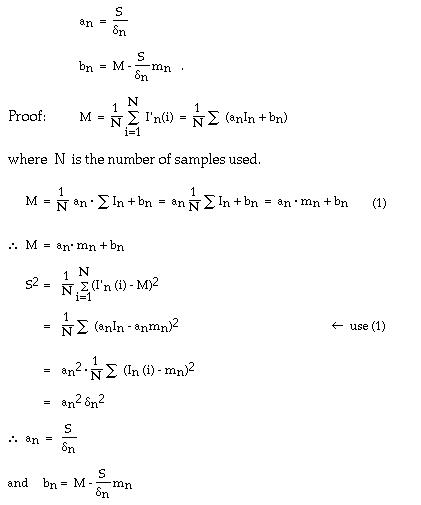
I'n = anIn + bnwhere I'n is the calibrated intensity and In is the original intensity
an and bn are the gain and bias to be determined.
The solution is:
For an 8-bit image, you may try to use M = 128 and S = 50 or may use the mean and standard deviation calculated from the entire sample.
This may not always work. The assumption behind this strategy is that detector responses are linear.
(2) Balance histogram
The assumption for balancing histogram is that each detector has the same probability of seeing the scene and, therefore, the grey-level distribution function should be the same. Thus if two detectors have different histograms (a discrete version of grey-level distribution function), they should be corrected to have the same histogram.
This is usually done by comparing their cumulative histograms as shown in Figure 5.4.
Figure 5.4. Balancing the histogram F2 to the reference histogram F1.
This process is done for each given grey level, g2, to find its cumulative frequencies fc2(g2) in F2. Then in F1 find the grey-level value, g1, such that its cumulative frequency fc1(g1) = fc2(g2). Then assign g1 to g2 in the histogram to be adjusted.
![]()
![]()
![]()
![]()
![]()
![]()
![]()
![]()
![]()
![]()
![]()
![]()
![]()
![]()